Python quick start - Part 1

The best way to understand python is to start using it. We will use here ipython, which is an advanced terminal that has many interesting features for scientific computing.

To start ipython open a terminal (in windows go to Start -> Run and type cmd) and type:

ipython

Python as calculator

You can first start using python as a calculator. Try the following:

# Simple addition
In [1]: 1+1
Out[1]: 2

# Powers
In [2]: 2**10
Out[2]: 1024

# Integer division. This will return only the quotient of the division
In [3]: 10/4
Out[3]: 2

# If you divide an integer by a float (decimal) number (in this case 4.0)
# you will get the full division.
In [4]: 10/4.0
Out[4]: 2.5

Numbers, and the results of your calculations can be stored in variables:

In [5]: a = 5

In [6]: a**3
Out[6]: 125

Python handles also complex numbers:

In [7]: a = 1 + 4j

In [8]: b = 3 - 2j

In [9]: c = a*b

In [10]: c
Out[10]: (11+10j)

You can get the real and imaginary part of your results easily:

In [11]: c.real
Out[11]: 11

In [12]: c.imag
Out[12]: 10

Note

Using the dot after anything in python, like you did in c.real for example, lets you explore a subpart of that thing, in a way, lets you look “inside” the thing you are using.

Python and arrays

Python’s mathematical capabilities are great, but there are a lot missing. To really use python for computations your will need to import numpy:

>>> import numpy

Note

From now on, we will avoid writing the “In [ ]:” part before input for brevity. We will put >>> in front of your input.

Now you can use many useful functions that are included in numpy by typing numpy.<function_name>:

>>> numpy.exp(10)
22026.465794806718

>>> numpy.log10(100)
2.0

The core of numpy are numerical arrays that allow you to perform fast calculations:

# You can create an array like this
>>> a = numpy.array([1,2,3])
>>> a
array([1, 2, 3])

Now a is array that can be manipulated:

>>> a**3
array([ 1,  8, 27])

You can create a list of numbers faster using the arange function:

>>> b = numpy.arange(10.0)

You can do even more complex calculations like \(b^3 - \frac{10}{b + 5} + 5\)

>>> c = b**3 - 10/(b + 5) + 5

Plotting

We can plot our arrays by using the matplotilb module. It is a very feature-full module that, lucky for us, has a set of convenient commands that make plotting easy. We will use only this subset of commands to start using matplotlib type:

from matplotlib import pyplot as plt

Don’t worry if you don’t understand this. In sort, inside matplotlib exists a submodule that is called pyplot. We import this and give it the name “plt” for convenience.

Now try the following:

# Create the plot based on c
>>> plt.plot(c)

# Show it on screen
>>> plt.show()

This should put the values of the c array in the y axis. Let’s try something more interesting:

# Get an array of numbers from -10 to 10
>>> x = numpy.arange(-10.0, 10.0)

# Calculate a more complicated y
>>> y = numpy.sin(x) * x**3

# Now plot y versus x
>>> plt.plot(x,y)

# Show the results
>>> plt.show()

(Source code, png, hires.png, pdf)

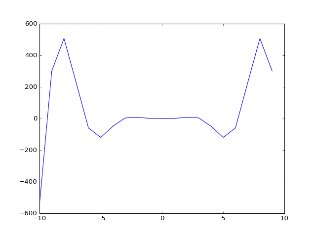
This should give you a plot, that looks very rough. This is because we are plotting only on integer numbers. We can improve this by using the numpy command “linspace” that can give you linearly spaced numbers. Close the previous plot and try:

# Get an array of 1000 numbers from -10 to 10
>>> x = numpy.linspace(-10.0, 10.0, 1000)

# Calculate a more complicated y
>>> y = numpy.sin(x) * x**3

# Now plot y versus x
>>> plt.plot(x,y)

# Show the results
>>> plt.show()

(Source code, png, hires.png, pdf)

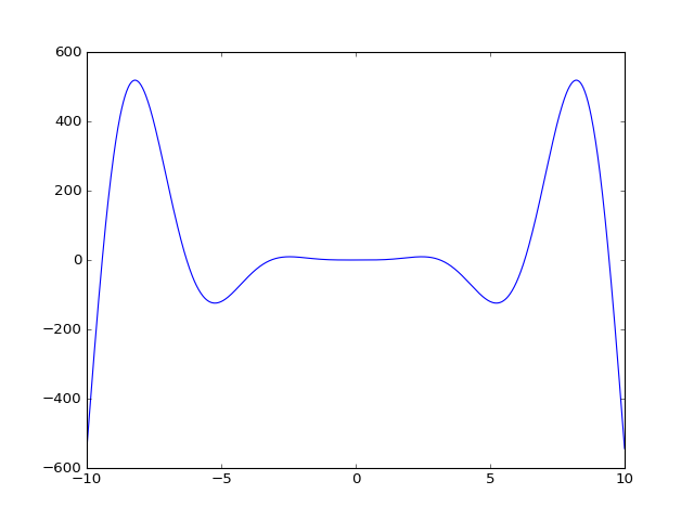
This looks much better!